The Logic of Exploratory and Confirmatory Data Analysis

Elissaios Karageorgiou

Brain Sciences Center, Veterans Affairs Medical Center, Minneapolis, MN

Department of Neuroscience, University of Minnesota Medical School, Minneapolis, MN

Neurology Department, University of Minnesota Medical School, Minneapolis, MN

Email: karag001@umn.edu

Accepted: February 10, 2011

KEYWORDS

diagnostic test assessment, exploratory data analysis, confirmatory data analysis, selection bias; biomarkers

ABSTRACT

Exploratory Data Analysis (EDA) and Confirmatory Data Analysis (CDA) are two statistical methods widely used in scientific research. They are typically applied in sequence: first, EDA helps form a model or a hypothesis to be tested, and then CDA provides the tools to confirm if that model or hypothesis holds true. When both analyses are applied within a single experiment, two main types of errors can occur that fall under the general term of selection bias. One error is the biased selection of the set of data used to confirm the model derived by the EDA. The other error occurs when CDA becomes part of EDA instead of being applied after EDA completion. As a result of selection bias, overfitting of a model can occur in a manner that makes the model stand true only narrowly, i.e. for the specific sample from which it was derived, without any generalizability. This bias in planning the analysis occurs frequently in the literature. This paper provides the theoretical background and the conceptual tools by which to identify such errors in the literature and to carry out the analysis properly. Applications of EDA and CDA in medical biomarker research are used as paradigms for clarification of concepts.

(Science is affirmed knowledge through logical arguments.)
Theaetetus, Plato

INTRODUCTION

Medical research has been increasingly focused on the development of biomarker models. According to Eykhoff (1974), a model is a representation of the essential aspects of an existing system (or a system to be constructed) which presents knowledge of that system in usable form. As such, biomarker models should sufficiently represent a person's biological state and ideally (a) improve and accelerate disease diagnosis, (b) substitute the current diagnostic gold-standard if too invasive, expensive, or time consuming, (c) allow follow-up of disease progression, and (d) substitute primary endpoints in clinical drug trials (De Gruttola et al. 2001). In clinical neuroscience, biomarkers may refer to a range of variables, from neuropsychological scores, to imaging variables, to biological substances. In this paper the more general term biomarker models, or simply models, will refer to any number of neural biomarkers and their combinations.

The Early Detection Research Network (http://edrn.nci.nih.gov) for development of cancer biomarkers has proposed a phase-design for potential clinical biomarkers, much like the phase-design of drug trials. Under this design, a model is first developed (Phase 1) and subsequently evaluated through case-control validation (Phase 2), retrospective preclinical validation (Phase 3), prospective preclinical evaluation (Phase 4), and disease control and burden reduction (Phase 5) (Pepe 2005). This is a robust evaluation method of a potential biomarker model and, ideally, should be pursued before introducing a model in everyday clinical practice. However, it is a costly and time consuming process and does not address the fact that an initial estimate of future error can be obtained while a model is being developed, thus avoiding testing a probably bad model in Phases 2 through 5. To obtain the error estimate of a biomarker model under development, researchers increasingly perform Exploratory Data Analysis (EDA) on a dataset and try to obtain confirmatory results on hypotheses derived from the EDA. In other words, they try to estimate whether the model derived from a selection process is accurate for the general population when modeled to be accurate for a specific dataset. Under this framework, creating a biomarker model is a necessary first step, but at the same time an error estimate of how the model will perform in the future is required. Now, a confirmatory estimate can be obtained by performing Confirmatory Data Analysis (CDA) but there are certain rules to be taken into consideration. A common violation of these rules is caused by selection bias, which results in the distortion of statistical inferences due to a biased collection of samples (Wikipedia contributors 2008). This, among many problems, may lead to overfitting the derived model, which means satisfying accuracy only for the specific dataset, thus preventing generalization. Indeed, 42% of recently published manuscripts on fMRI in high-impact journals were found to have some sort of selection bias in their analysis with an additional 14% possibly containing such a bias (Kriegeskorte et al. 2009).

In what follows the basic concepts behind EDA and CDA will be initially presented to clarify the role of each in biomarker development. Then, the two most commonly applied plans for biomarker model development and error estimation will be outlined (Separate-sample vs. Single-sample), followed by a clarification of differences between Internal and External Cross-Validation. Then, the most common pitfalls in biomarker model development and some rules to identify and prevent them will be discussed. Finally, scientific reasoning principles will be outlined and selection bias will be explained as an instantiation of logical fallacy.

CONFIRMATORY vs. EXPLORATORY DATA ANALYSIS

Confirmatory Data Analysis

Traditionally, statistics in medicine have been used to evaluate a preconceived hypothesis. Tests applied for this purpose fall under CDA and reflect the majority of statistical analyses in research (e.g. a t-test in evaluating treatment effect), keeping in mind that confirmation in classical statistics (Fisherian and Neyman-Pearson schools) is based on rejecting the null hypothesis (i.e. that something is not true), rather than accepting a hypothesis (see Sokal and Rohlf 1995). A specific application of CDA in medical research could be to test whether a particular biomarker differs significantly between healthy controls and patients, to determine whether a specific intervention significantly changed the prognosis of a group of patients relative to another intervention, etc. When the hypothesis preexists (e.g. a specific biomarker model or a specific drug) from a prior independent study, then evaluation simply requires a straightforward CDA. However, in cases where no specific hypothesis exists, then one has to be developed through EDA before CDA is pursued.

Exploratory Data Analysis

EDA is a term coined by Tukey (1977) to encompass ways of graphically and quantitatively analyzing data to help derive a hypothesis to be tested. However, EDA is more than graphing data, it is an attitude and a flexibility (Tukey 1980), and any activity leading to a testable hypothesis can be considered EDA. Here, I use this broader definition of EDA. Hypothesis building is achieved by inductively developing a hypothesis for the general population based on observations from a specific sample and prior theoretical knowledge. The inherent flexibility in EDA allows a wide range of techniques to be used, and is not as confined as the methods applied in CDA; however, statistical techniques applied in CDA can be used in EDA, as long as their use lies in building a hypothesis. For example, all algorithms that are employed to develop biomarker models through a selection process can be considered EDA techniques, since they help develop a hypothesis for a model's value in clinical practice. In general, EDA is an inductive decision process, whereas CDA is a deductive evaluation process. Each one provides the statistical tools to answer a specific scientific question. When the scientific issue is to build a hypothesis (e.g. decide which biomarkers to select in developing a potentially good model), EDA should be used; when the issue is to verify that hypothesis (e.g. by evaluating the goodness of the developed model), CDA should be used.

DATA ANALYSIS plans for biomarker model development and error estimation

Separate-sample plan

The most robust approach to evaluate a specific biomarker model's performance is to first develop the model using EDA on a training set of subjects and then use CDA to evaluate that model on a separate test set of subjects (Fig. 1a) (Ambroise and McLachlan 2002). The development of the model entails two aspects: (a) the selection of relevant biomarkers from a pool of many (also called feature selection), and (b) fine-tuning of biomarkers, either by weighting their coefficients or setting their normal limits within confidence intervals (CI). For example, the differential weighting of coefficients can be seen in models where a number of neuropsychological scores are used to characterize disease severity or predict disease progression; CIs are commonly seen in all aspects of research.

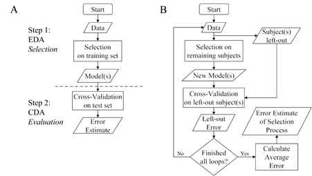Figure 1. Data analysis plans for biomarker model development and error estimation. (A) Separate-sample plan with EDA and subsequent error estimation using CDA. Any data analysis plan, that also evaluates produced model(s), must first develop the model(s) and then separately evaluate the model(s) produced. (B) Single-sample plan error estimation. In a single-sample plan, first one or more subjects are left out and then a model is developed on the remaining subjects. The model is then evaluated on the left-out subject(s). The process is repeated, each time resetting the left-out subject(s). The error estimate of the selection algorithm is the average error from all loops.

In the case where EDA provides several alternative models instead of a single one, all models must be evaluated through CDA and their combined error rate reported, rather than selectively reporting individual errors of the best models. This might seem counterintuitive, since the goal is to retain a good model. However, model development stops with EDA. CDA cannot be used to aid in biomarker model development; it is only used to provide model error estimates. The use of an individual model's error rate on a new set of subjects, in order to further accept or reject the model, falls under EDA, and is in no way a confirmatory test. Implications concerning improper planning and separation of EDA and CDA will be discussed more extensively in the following sections with an emphasis on Cross-Validation (CV) and on detecting pitfalls in model development.

Consider the following separate-sample example. A group of researchers wishes to find the single best protein in the cerebrospinal fluid (CSF) that can help in diagnosing multiple sclerosis. Since at the initiation of the study there is no specific protein considered as the best biomarker, one has to be identified first on a training set of subjects; in other words, a hypothesis must be built through EDA. One approach to this end might entail performing linear discriminant analysis (LDA) between patients and controls using each one of the proteins found in CSF as the predictor. The protein that yields the best discrimination of the two groups can be retained as the possible best biomarker. Now that the hypothesis has been developed, the researchers will need to evaluate it through CDA. In the separate-sample plan this can be achieved by using the discriminant coefficients that were derived from the EDA to classify a new test set of patients and controls. The error in the test set will reflect the diagnostic accuracy of the specific CSF protein in the general population.

Single-sample (loop) plan

This type of plan is useful when there are not enough subjects to allow for the development of a model and its evaluation using separate training and test sets. This occurs frequently when using data from few subjects relative to the total number of variables. In this case, the researcher needs to use all the subjects in the dataset to retain the maximum amount of information for model development, but a different error estimation approach from the one described above has to be taken. The question is how to evaluate the selection process, since all subjects are required for the EDA. Tukey (1980) addressed this problem in its more general form when assessing EDA significance, and proposed the use of the jackknife as a solution. With the jackknife (also called leave-one-out CV), a single case is left-out at the very beginning, then models are developed according to EDA, and the errors of the models are estimated by testing on the case left-out. This process is repeated iteratively until all subjects are left out of the EDA once. The overall error rate is the average error rate from all iterations (Fig. 1b). It is important to note that through this process no single model is produced. Instead, in each loop, one or more different models are developed both for the biomarkers selected and the coefficients/CI these biomarkers carry, since the training set from which the model is derived is different each time (by one subject). The purpose of this approach is to provide an error estimate for the entire search algorithm, given a sample of subjects. It is not specific to any single result, but can give an unbiased estimate of future model performance if all subjects were to be used in developing a model (Ambroise and McLachlan 2002). In contrast, a robust approach to evaluate a specific model derived by an algorithm is by cross-validating that model on a totally separate test set of cases through a separate-sample plan.

There are variations of the jackknife. The most popular approaches include the K-fold CV, in which more than one subject is left out in each loop, and the bootstrap (Efron and Tibshirani 1993). These approaches provide a slightly more biased error estimate, but with reduced variability, mainly due to more subjects being left-out (Ambroise and McLachlan 2002). Irrespective of the CV approach adopted, the basic concepts remain the same: in each loop a model is developed on the training set of subjects, and then that model is evaluated on the left-out test-subjects, with the error estimate being the average error from all loops.

As an example of a single-sample plan, consider a voxel-based-morphometry study where a group of researchers tries to develop a biomarker model for diagnosing Alzheimer's disease using a combination of pertinent voxels. A stepwise-LDA is applied for biomarker model development, which reflects the EDA part of the experiment. Since there are thousands of variables (i.e. voxels) and relatively few subjects, a leave-one-out CV is applied to retain maximum information for model development and, at the same time, to estimate future performance of a derived model. In each loop, a new stepwise-LDA is performed which leads to a new model composed from a different combination of voxels and coefficients each time. Each left-out subject is classified according to the model of the respective loop. The overall classification of subjects and the evaluation of the derived sensitivity and specificity reflect the CDA part of the experiment.

INTERNAL vs. EXTERNAL CROSS-VALIDATION

Cross-validation refers to the evaluation of a model derived from a training set of subjects on a second sample set (Duda et al. 2001). When the results obtained are used only to report prediction error estimates, the CV is called External (ECV), and the second sample is a true test set. If the error obtained from the second sample is used to select the best of the derived models, then the CV is called Internal (ICV), because it is part of model development, and the second sample is a second training set. Thus, ICV can lead to erroneous conclusions if one refers to its results as error estimates. In contrast, ECV provides an unbiased error estimate of a model (Ambroise and McLachlan 2002). ICV and ECV can be applied to either separate-sample or single-sample plans.

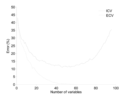Figure 2. Comparison between ICV and ECV. Sequential linear discriminant analyses were performed on an artificial two group dataset of 100 subjects by introducing new variables which individually contain minimal discriminatory information.

To clarify differences between ICV and ECV, Fig. 2 provides error rates from an artificial dataset by introducing increasing numbers of variables in a model for a fixed number of subjects. The ICV results consistently improve whereas the ECV results reach a plateau and then worsen. The decreasing ICV error rate indicates overfitting, where undue emphasis is placed on information that is specific to the particular dataset. This can occur when too many variables, relative to the number of subjects, are introduced in the model, or when a selection algorithm chooses variables specifically to maximize group discrimination, and would thus use dataset-specific information. If the ICV-selected models were to be used on a new sample set, the error rate would probably be worse than the respective ECV.

DETECTING PITFALLS IN MODEL DEVELOPMENT

Given the guidelines above, it is straightforward to correctly combine EDA and CDA, and interpret the results. However, researchers often reach incorrect conclusions because of a selection bias when defining training or test samples. With this in mind, there are certain pitfalls one has to avoid when planning an experiment or reaching conclusions, as follows.

Separate-sample plan with ICV but without subsequent ECV

A common error is the development of models based on results from an ICV process without verifying those results through an ECV process. Usually authors will report something similar to:

“The search algorithm was run on a training set of subjects and several models were produced… Those models were subsequently tested on a test set of subjects and the error rate evaluated… The final models chosen are the ones that minimize the total error in cross-validation.”

The bias in this case lies in the fact that selection was not based solely on the initial training set, but also on the error rate of the test set (ICV), which practically became a second training set (Fig. 3a). A variation to the above is obtained when there is no search algorithm, and all possible solutions are evaluated. For example, this is the case when evaluating each voxel's classification potential in an MRI experiment and then selecting the best voxels based on a test set of subjects. Such erroneous conclusions concern not only incorrect biomarker model development for disease diagnosis, but also incorrect statements in basic neuroscience regarding brain function, an area subject to less scrutiny. It should be noted that this type of error does not necessarily mean that the results presented will not hold true for new subjects, but it does not provide proof of the researchers' statements. Usually, if the number of good models produced is close to chance levels, then the statements made will probably be false. This process will lead to overfitting of the model, making the model hold true only for the specific dataset.

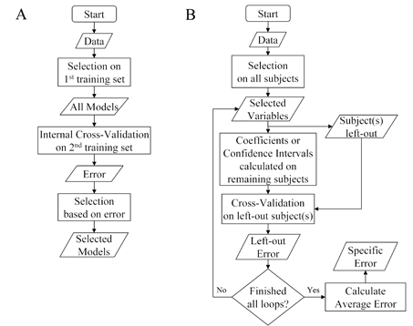Figure 3. Common pitfalls in data analysis plans. (A) Model development under ICV without subsequent error estimation. In this case model development is based on an initial selection algorithm and the error estimate from an ICV. Unless a new error estimate on a new set of subjects is evaluated, then no truly predictive error estimation is provided of the final models. Compare to figure 1A. (B) Selection bias in a single-sample plan. A common mistake in a single-sample plan is made when the feature selection process precedes leaving out any subject(s). In this case the selection is biased because all subjects' data were used in feature selection and thus provide a specific model's error, rather than an error for the selection process as a whole. Compare to figure 1B.

Selection bias in a loop plan

Selection bias is observed more often when error estimates of a model are obtained through a single-sample plan. Most mistakes made in the literature are related to using the same subjects' data for both training and CV of a model. As mentioned above, model development is both a feature selection process and a coefficient/CI weighting process. If, for example, a researcher tries to develop a model of neuropsychological scores that predicts progression of disease Q in a number of years, first the appropriate scores from a list of several should be selected and then the correct coefficients/CI on each selected score should be applied. If the researcher's statement reads like,

“The search algorithm was run and the ideal variables were selected… The error estimate was subsequently evaluated by a leave-one-out cross-validation,”

this implies that all subjects' data were used to select pertinent variables, and the loop procedure was only used to evaluate the goodness of setting coefficient/CI weights on those variables (Fig. 3b). However, the coefficient/CI weighting is also biased, since the variables are usually selected to provide good weights for all subjects as well. If, on the contrary, a researcher had a specific subset of variables in mind (e.g. from prior results on a different sample), and if all these variables were used in a single model, then a loop as above would be appropriate, since no selection of variables would have taken place. An easy way to spot such a mistake is by determining if the researcher reports an error estimate for a specific model, or for the search algorithm as a whole. Since a loop plan can only provide an error estimate for the entire selection process, mentioning a specific model's error is incorrect. Finally, similar mistakes can be made when using commercial statistical packages. Such packages have selection techniques, usually stepwise, that first use all subjects' data to select variables and then use a loop approach for CV. Thus, if a researcher is not aware of this fact, he or she will reach the wrong conclusions.

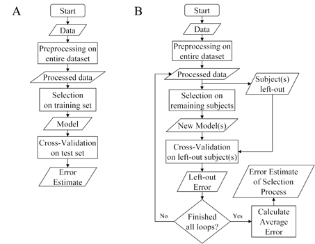Figure 4. Selection bias when preprocessing data. Selection bias can be induced by preprocessing data from (A) both training and test sets in a separate-sample plan, or (B) data from all subjects in a single-sample plan. In the separate-sample plan only the training set's data should be preprocessed and, based on the parameters they provide, have the test set's data transformed. In the single-sample plan, preprocessing should occur in each loop on the left-in subjects and from the produced parameters the left-out subjects' data transformed.

Selection bias by preprocessing data

A more subtle error made with less obvious effects is the preprocessing of the original data based on information from all subjects' data. This error can either occur in a separate-sample (Fig. 4a) or a single-sample plan (Fig. 4b). For example, a researcher might want to first transform subjects' data and then perform the main modeling algorithm. Two common examples of data transformation are standardization, which makes between-variable contributions comparable, and Principal Component Analysis (PCA), which reduces the dimensions (i.e. variables used) of the dataset at hand while retaining most of the data's information (Duda et al. 2001). In such cases, only the subjects of the training set should contribute in obtaining a transformed distribution. Commonly, researchers transform the entire dataset, including the test subjects. As an example, consider an fMRI experiment where there are thousands of voxels that can be incorporated in the analysis. Researchers might apply PCA across subjects to reduce the number of variables prior to applying their modeling algorithm. The mistake becomes apparent when one considers how a new subject will be evaluated in the future. Since that subject did not contribute to the preprocessing, it should have its data transformed according to the subjects that were in the original study. That same rule applies for the test-set subjects, or left-out subjects, of the study.

FINAL REMARKS

The goal of this paper was to bring into focus the logic of data analysis and model-building by helping researchers to avoid, and readers to detect, common mistakes during EDA and CDA modeling. To provide theoretical rigor beyond simple do and don't, model development and evaluation were presented through the perspective of combining EDA and CDA. The clear separation of these two processes allows for a properly conducted study with accurate interpretation of results. Under the general rules of EDA and CDA, separate-sample and single-sample plans were described. Common pitfalls were presented based on the type of plan, but combinations and variations of those also exist. The theoretical background presented provides the necessary conceptual tools to evaluate whether data analysis was properly planned and whether conclusions reached are correct.

In general, when evaluating a study that involves both a selection and an evaluation process, as in biomarker model development, it is advisable to confirm that EDA and CDA are truly separate, and in case the methodology is unclear, to rephrase it to explicate these two types of analysis. Alternatively, one can also determine if test subjects in the separate-sample or loop plan were treated as a new subject would have been treated after finalizing a model.

Finally, a robust and possibly the only way to evaluate a specific model's future performance is through an ECV on a totally new test set of cases after all model parameters are fixed. In a way, this is analogous to clinical drug trial phases and the design format proposed by the Early Detection Research Network for development of cancer biomarkers (Pepe 2005).

ACKNOWLEDGMENTS

Thank you to Dr. Siamak Noorbaloochi for reviewing the manuscript prior to submission.

REFERENCES

Ambroise C, McLachlan GJ (2002) Selection bias in gene extraction on the basis of microarray gene-expression data. Proc Natl Acad Sci U S A 99: 6562-6566

De Gruttola VG, Clax P, DeMets DL, Downing GJ, Ellenberg SS, Friedman L, Gail MH, Prentice R, Wittes J, Zeger SL (2001) Considerations in the evaluation of surrogate endpoints in clinical trials: summary of a National Institutes of Health Workshop. Control Clin Trials 22: 485-502

Duda RO, Hart PE, Stork DG (2001) Pattern classification, 2nd edn. Wiley-Interscience, New York, NY

Efron B, Tibshirani RJ (1993) An introduction to the bootstrap. Chapman & Hall, New York, NY

Eykhoff P (1974) System identification: parameter and state estimation. Wiley & Sons, Chichester, UK

Kriegeskorte N, Simmons WK, Bellgowan PS, Baker CI (2009) Circular analysis in systems neuroscience: the dangers of double dipping. Nat Neurosci 12: 535-540

Pepe MS (2005) Evaluating technologies for classification and prediction in medicine. Stat Med 24: 3687-3696

Sokal RR, Rohlf FJ (1995) Biometry, 3rd edn. W. H. Freeman and Company, New York, NY

Tukey JW (1977) Exploratory data analysis. Addison-Wesley, Reading, MA

Tukey JW (1980) We need both exploratory and confirmatory. Am Stat 34: 23-25